Visualizing atomic type orbitals in molecules

How to compute and visualize natural atomic orbitals with PySCF

Introduction

Sometimes we need to display atomic type orbitals in a schematic way to visualize simple concepts. The molecular orbitals or even localized orbitals are then overly complex. Simple examples are the ChemDraw-style orbitals, which are used to rationalize reactions in organic chemistry. Now, is it possible to obtain similar orbitals, but in 3D?

Computing the 3D structure

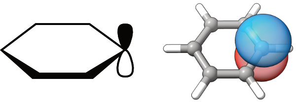
We will use benzene as an example. First we generate the 3D coordinates using RDKit

from rdkit import Chem
from rdkit.Chem import AllChem

smiles = "c1ccccc1"
mol = Chem.MolFromSmiles(smiles)
mol = Chem.AddHs(mol)
mol

AllChem.EmbedMolecule(mol)
AllChem.MMFFOptimizeMolecule(mol);

We visualize the structure using py3Dmol

import py3Dmol

v = py3Dmol.view()
v.addModel(Chem.MolToMolBlock(mol), 'mol')
v.setStyle({'stick':{}});

Calculating the NAOs

We will now use PySCF to calculate the NAOs. As we are only interested in the schematic form of the orbitals, the small STO-3G basis set will be sufficient. First we construct the PySCF Mole object from the RDKit Mol object.

import pyscf
from pyscf import gto, lo, tools, dft 

elements = [atom.GetSymbol() for atom in mol.GetAtoms()]
coordinates = mol.GetConformer().GetPositions()
atoms = [(element, coordinate) for element, coordinate in zip(elements, coordinates)]

pyscf_mole = gto.Mole(basis="sto-3g")
pyscf_mole.atom = atoms
pyscf_mole.build();

We then run the DFT calculation, which is actually quite fast

mf = dft.RKS(pyscf_mole)
mf.xc = 'b3lyp'
mf.run();

converged SCF energy = -229.251421996489

We can now compute the NAOs from the 1-st order reduced density matrix. Note that we are here actually calculating the pre-orthogonal NAOs (PNAOs) that are even more local that the NAOs. We the write the PNAOs to cube files - these files can be quite large, ca 3 MB each.

dm = mf.make_rdm1()
naos = lo.nao.prenao(pyscf_mole, dm)

for i in range(naos.shape[1]):
    tools.cubegen.orbital(pyscf_mole, f'benzene_nao_{i+1:02d}.cube', naos[:,i],  nx=60, ny=60, nz=60)

Visualizing the NAOs

Here we use py3Dmol and ipywidgets to interactively view the orbitals.

def draw_orbital(view, i):
    with open(f"./benzene_nao_{i:02d}.cube") as f:
        cube_data = f.read()
    view.addVolumetricData(cube_data, "cube", {'isoval': -0.04, 'color': "red", 'opacity': 0.75})
    view.addVolumetricData(cube_data, "cube", {'isoval': 0.04, 'color': "blue", 'opacity': 0.75})
    view.addModel(Chem.MolToMolBlock(mol), 'mol')
    view.setStyle({'stick':{}})
    view.zoomTo()
    view.update()
    view.clear()

view = py3Dmol.view(width=400,height=400)
view.show()
draw_orbital(view, 25)

You appear to be running in JupyterLab (or JavaScript failed to load for some other reason). You need to install the 3dmol extension:
jupyter labextension install jupyterlab_3dmol

Interactive viewing

Unfortunately, the interactive viewer doesn’t display on the blog. Try running the code below on Binder or locally on your machine.

from ipywidgets import fixed, interact_manual

n_orbitals = naos.shape[1]
view = py3Dmol.view(width=400,height=400)
view.show()
interact_manual(draw_orbital, view=fixed(view), i=(1, n_orbitals));

You appear to be running in JupyterLab (or JavaScript failed to load for some other reason). You need to install the 3dmol extension:
jupyter labextension install jupyterlab_3dmol

Acknowledgements

iwatobipen’s blog post on the rendering of orbitals with py3Dmol was very helpful when writing this notebook.

Reuse

Code free to use under an MIT license. For citation, use webpage address and access date.