Frontier molecular orbitalets

How to compute and visualize orbitalets with PySCF

Introduction

A recent article in Chemistry World caught my attention. It reported the recent work by Yang and co-workers on describing chemical reactivity with so-called orbitalets. Orbitalets are a type of localized molecular orbital that came out of the Yang group’s work on eliminating the delocalization error from density functionals. The highest occupied orbitalet is called the HOMOL, and the lowest unoccupied orbitalet is called the LUMOL.

Orbitalets can be seen as an intermediate between the fully delocalized canonical molecular orbitals (CMOs) and fully localized orbitals (LOs). As such, their energies are fairly close to the CMOs, while their localized character allows easier interpretation of reactivity in terms of frontier molecular orbital theory (FMO). Regular localization schemes like Foster-Boys, Natural Bond Orbitals loose the connection to the CMO energies, and therefore the resulting LOs are more difficult to relate directly to reactivity. The orbitalets represent some type of compromise, although it remains to be seen how well they work in practice, over a large range of different compounds and reactivity patterns.

When I read an article like this, I immediately look for code that would enable me to try the method myself. Luckily, the authors have also published an article about LibSC, a library that can calculate orbitalets. It features a Python interface that can be used with either Psi4 or PySCF. Here we will try out the PySCF interface.

Orbital

Orbitalet

Figure 1: Orbital vs. orbitalet.

Installation

LibSC needs to be installed from source, and we need to have the following on our system

• C++ and C compilers
• The Eigen library
• CMake
• OpenMP
• GNU Make or Ninja

To use the Python interface to PySCF, we also need to have these installed:

• PySCF
• NumPy

I followed the installation instructions approximately. On my Mac, I would use

$ CC=gcc-11 CXX=g++-11 cmake -B build -DCMAKE_BUILD_TYPE=Release
$ cmake --build build -j 8 

If everything goes well, the build/src directory then needs to be added to the system path to allow import of the pyscf_losc module.

Calculating the orbitalets

import sys
sys.path.insert(0, "/Users/kjelljorner/bin/losc/build/src")
import os

import py3Dmol
import pyscf
import pyscf_losc
from morfeus.conformer import _add_conformers_to_mol
import polanyi
from polanyi.workflow import opt_xtb
from pyscf import tools
from rdkit import Chem
from rdkit.Chem import AllChem

os.environ["OMP_NUM_THREADS"] = "4" # Adjust to how many processors you want PySCF and LibSC to use
polanyi.config.OMP_NUM_THREADS = "4"

First we generate coordinates for the molecule with RDKit and then optimize using GFN2-xTB. Here we use a convenience function from the polanyi package, soon to be released. The geometry refinement step with xtb can probably be skipped for illustration purposes.

# Generate the molecule with RDKit
smiles = "C/[N+](=C/C1=CC=CC=C1)/[O-]"
mol = Chem.MolFromSmiles(smiles)
mol = Chem.AddHs(mol)
AllChem.EmbedMolecule(mol)
AllChem.MMFFOptimizeMolecule(mol)

# Optimize with xtb
elements = [atom.GetSymbol() for atom in mol.GetAtoms()]
coordinates = mol.GetConformer().GetPositions()
opt_coordinates = opt_xtb(elements, coordinates)

# Add the optimized coordinates back to the Mol for later visualization
mol.RemoveAllConformers()
_add_conformers_to_mol(mol, [opt_coordinates])

We then do a single-point calculation with PySCF. For illustration purposes, we use the small STO-3G basis set. For publication quality results, a larger basis set would of course need to be used. The PySCF calculation is quite fast, ca 7s on my computer.

# Create PySCF Mole object
atoms = [(element, coordinate) for element, coordinate in zip(elements, opt_coordinates)]
pyscf_mole = pyscf.gto.Mole(basis="sto-3g")
pyscf_mole.atom = atoms
pyscf_mole.symmetry = False  # turn off symmetry in PySCF
pyscf_mole.build()

# Conduct the DFA SCF calculation from PySCF.
mf = pyscf.scf.RKS(pyscf_mole)
mf.xc = "B3LYP"
mf.kernel();

converged SCF energy = -434.318630743168

We then calculate the orbitalets and their energies using LibSC.

# Configure LOC calculation settings.
pyscf_losc.options.set_param("localizer", "max_iter", 1000)

# Conduct the post-SCF LOC calculation
_, _, losc_data = pyscf_losc.post_scf_losc(
    pyscf_losc.BLYP,
    mf,  
    return_losc_data = True
)    

The orbital localization is not a cheap calculation and actually takes almost the same time as the SCF calculation, ca 8 s on my computer. We can now take a look at the orbitalet vs the orbital.

Visualize the orbitalets

We will use py3Dmol to draw the orbitals and write a small convenience function that will do the heavy lifting

def draw_orbital(view, mol, filename):
    with open(filename) as f:
        cube_data = f.read()
    view.addVolumetricData(cube_data, "cube", {'isoval': -0.04, 'color': "red", 'opacity': 0.75})
    view.addVolumetricData(cube_data, "cube", {'isoval': 0.04, 'color': "blue", 'opacity': 0.75})
    view.addModel(Chem.MolToMolBlock(mol), 'mol')
    view.setStyle({'stick':{}})
    view.zoomTo()
    view.update()
    view.clear()

We use PySCF to create cube files of the orbitals. We store both the HOMO, HOMOL, LUMO and LUMOL.

homo_idx = pyscf_mole.nelectron // 2 - 1
lumo_idx = homo_idx + 1
orbitalets = losc_data["C_lo"][0]
_ = tools.cubegen.orbital(pyscf_mole, f'orbitalet_homo.cube', orbitalets[:,homo_idx],  nx=60, ny=60, nz=60)
_ = tools.cubegen.orbital(pyscf_mole, f'orbital_homo.cube', mf.mo_coeff[:,homo_idx],  nx=60, ny=60, nz=60)
_ = tools.cubegen.orbital(pyscf_mole, f'orbitalet_lumo.cube', orbitalets[:,lumo_idx],  nx=60, ny=60, nz=60)
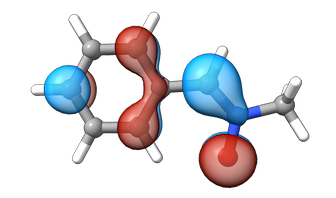
_ = tools.cubegen.orbital(pyscf_mole, f'orbital_lumo.cube', mf.mo_coeff[:,lumo_idx],  nx=60, ny=60, nz=60)

We can visualize the orbitals with py3Dmol. The HOMOL is significantly more localized than the HOMO.

view = py3Dmol.view(width=400, height=400)
view.show()
draw_orbital(view, mol, "orbital_homo.cube")

You appear to be running in JupyterLab (or JavaScript failed to load for some other reason). You need to install the 3dmol extension:
jupyter labextension install jupyterlab_3dmol

view = py3Dmol.view(width=400, height=400)
view.show()
draw_orbital(view, mol, "orbitalet_homo.cube")

You appear to be running in JupyterLab (or JavaScript failed to load for some other reason). You need to install the 3dmol extension:
jupyter labextension install jupyterlab_3dmol

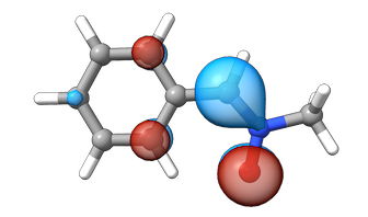
For the LUMOL, this localization becomes even more evident

view = py3Dmol.view(width=400, height=400)
view.show()
draw_orbital(view, mol, "orbital_lumo.cube")

You appear to be running in JupyterLab (or JavaScript failed to load for some other reason). You need to install the 3dmol extension:
jupyter labextension install jupyterlab_3dmol

view = py3Dmol.view(width=400, height=400)
view.show()
draw_orbital(view, mol, "orbitalet_lumo.cube")

You appear to be running in JupyterLab (or JavaScript failed to load for some other reason). You need to install the 3dmol extension:
jupyter labextension install jupyterlab_3dmol

I will leave it up to the reader to decide whether the HOMO/HOMOL and LUMO/LUMOL energies are “sufficiently” similar or not

print(f"HOMO (eV): {losc_data['dfa_orbital_energy'][0][homo_idx]:.3f}")
print(f"HOMOL (eV): {losc_data['losc_dfa_orbital_energy'][0][homo_idx]:.3f}")
print(f"LUMO (eV): {losc_data['dfa_orbital_energy'][0][lumo_idx]:.3f}")
print(f"LUMOL (eV): {losc_data['losc_dfa_orbital_energy'][0][lumo_idx]:.3f}")

HOMO (eV): -2.831
HOMOL (eV): -5.921
LUMO (eV): 1.425
LUMOL (eV): 4.198

Reuse

Code free to use under an MIT license. For citation, use webpage address and access date.